Conditional Formatting
Make your data colorful and easy to understand
Conditional Formatting
Conditional formatting automatically changes the color of cells based on their values.
Think of it like traffic lights:
- Green = Good
- Yellow = Warning
- Red = Problem
Excel does this automatically for you.
Why Use It?
Look at these two tables:
Without formatting: 85, 42, 91, 38, 76, 55, 88, 29
With formatting: You instantly see which numbers are high (green) and low (red).
It makes data easy to understand at a glance.
How to Apply Conditional Formatting
Step 1: Select the cells you want to format
Step 2: Go to Home tab
Step 3: Click Conditional Formatting
Step 4: Choose a rule (like "Greater Than")
Step 5: Set your value and color
Step 6: Click OK
Done. Excel will now color your cells automatically.
Example 1: Highlight High Sales
You have sales numbers. You want to highlight all sales above 1000.
- Select your sales data
- Home tab > Conditional Formatting > Highlight Cell Rules > Greater Than
- Type: 1000
- Choose: Green Fill
- Click OK
Now all sales above 1000 are green.
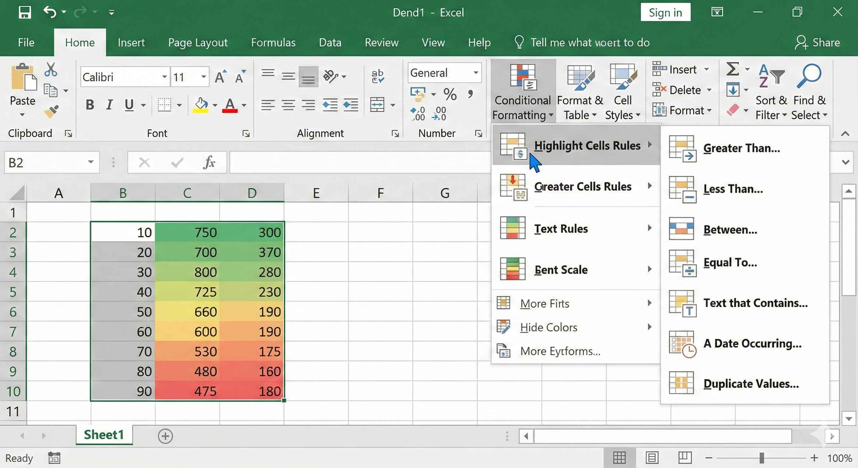
Example 2: Highlight Low Stock
You have inventory. You want to see which items are low (below 10).
- Select your stock numbers
- Home tab > Conditional Formatting > Highlight Cell Rules > Less Than
- Type: 10
- Choose: Red Fill
- Click OK
Now all items below 10 are red. You know what to reorder.
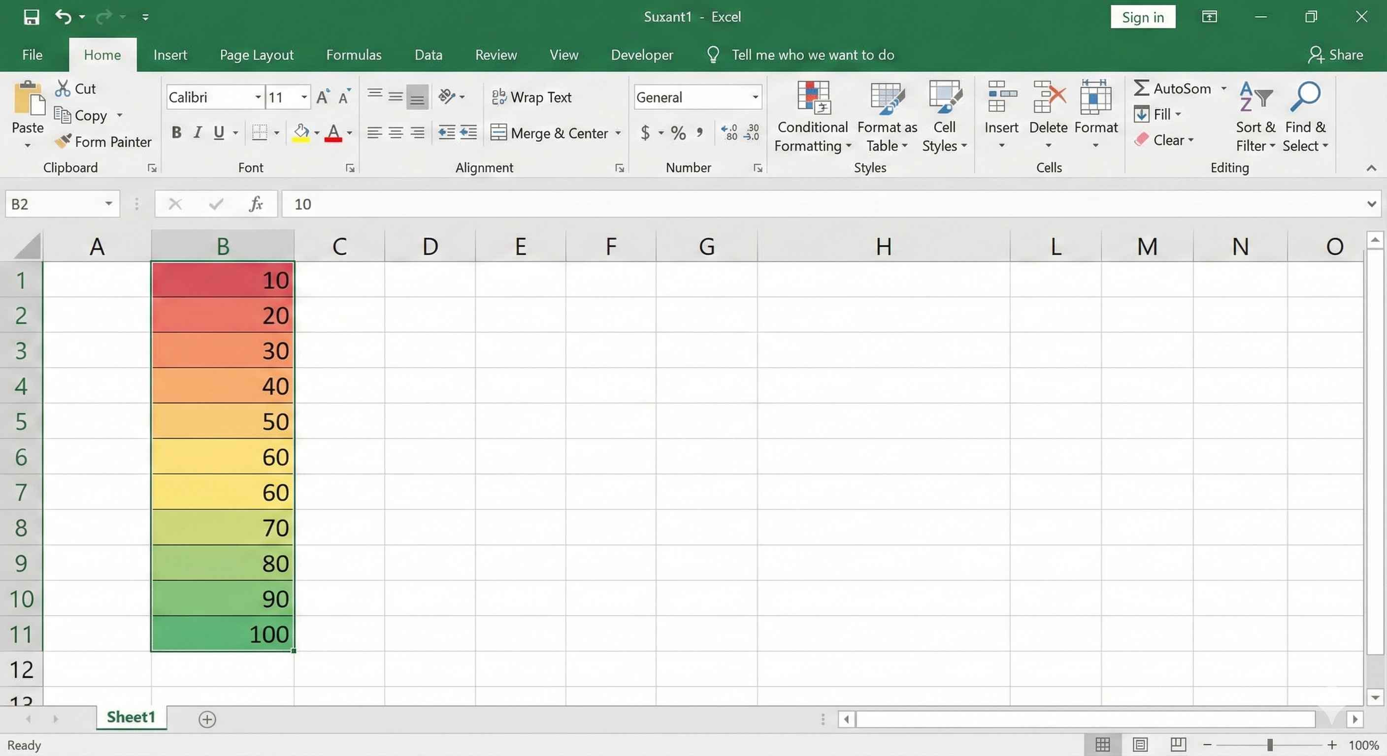
Example 3: Color Scale
Color scale shows a range of colors from low to high.
- Select your data
- Home tab > Conditional Formatting > Color Scales
- Pick a color scheme (Green-Yellow-Red)
Now your data shows:
- Lowest values = Red
- Middle values = Yellow
- Highest values = Green
Example 4: Data Bars
Data bars show mini bar charts inside cells.
- Select your data
- Home tab > Conditional Formatting > Data Bars
- Pick a color
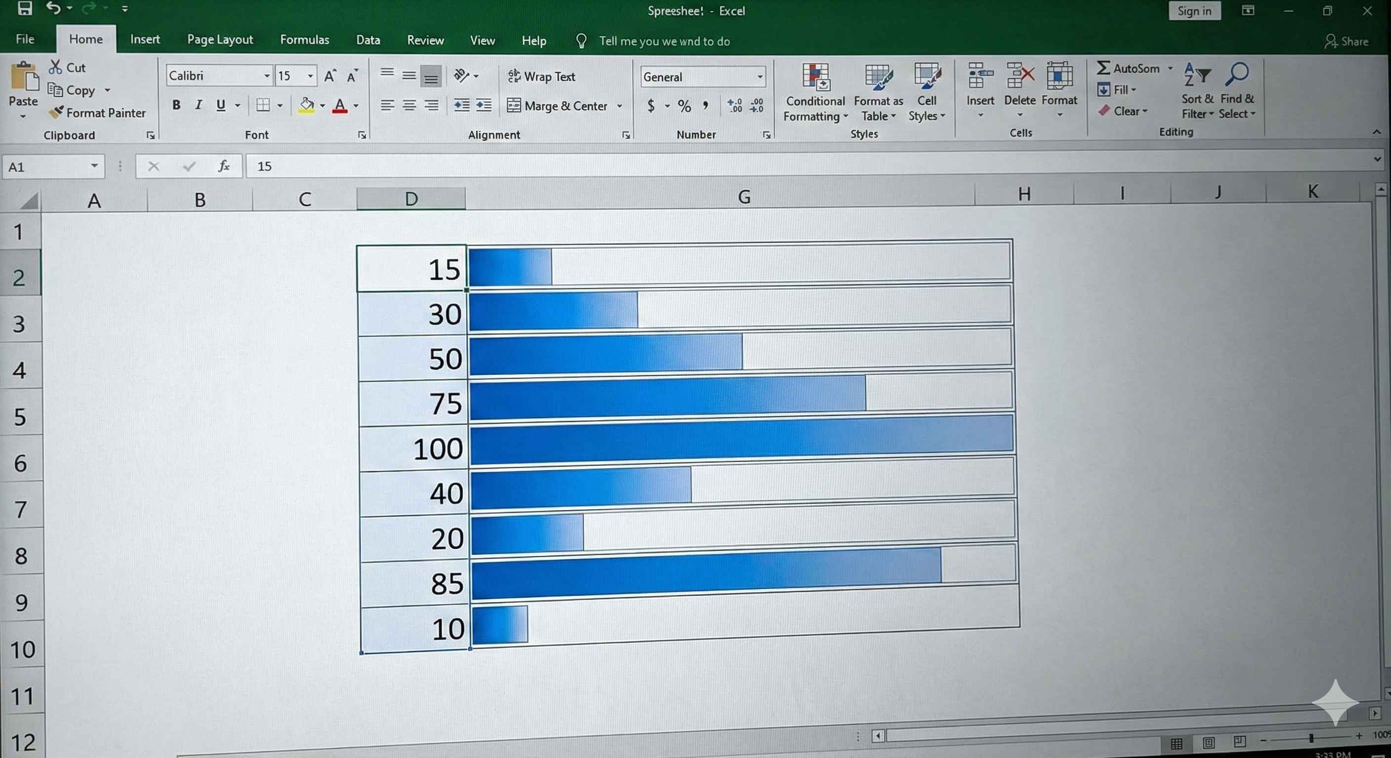
Now each cell has a bar. Longer bar = bigger number. You can compare values instantly.
Types of Conditional Formatting
| Type | What It Does | Use For |
|---|---|---|
| Highlight Cells | Colors cells based on value | Above/below a number |
| Top/Bottom | Colors top 10 or bottom 10 | Best/worst performers |
| Data Bars | Shows bars in cells | Comparing numbers |
| Color Scales | Gradient from low to high | Seeing patterns |
| Icon Sets | Shows icons (arrows, stars) | Status indicators |
Real Examples
Grades:
- Green: 90 and above (A)
- Yellow: 70-89 (B/C)
- Red: Below 70 (Fail)
Budget:
- Green: Under budget
- Red: Over budget
Sales:
- Data bars to compare salespeople
Inventory:
- Red: Stock below 10 (reorder)
- Green: Stock above 50 (good)
Tips
- Use 2-3 colors maximum. Too many colors are confusing.
- Green = Good, Red = Bad. Keep it simple.
- Test your formatting with different values.
Summary
- Conditional formatting colors cells automatically
- Makes data easy to read at a glance
- Home tab > Conditional Formatting
- Use for highlighting high/low values, comparisons, and patterns
- Keep colors simple and consistent
This is one of the most useful features in Excel for making professional reports.