PivotCharts
Turn your PivotTable into a visual chart
PivotCharts
A PivotChart is a chart that shows your PivotTable data visually.
PivotTable: Numbers in rows and columns PivotChart: Picture of those numbers
Charts are easier to understand. Instead of reading numbers, you see bars, lines, or pie slices.
Why Use PivotCharts?
- Numbers are hard to compare. Charts make it easy.
- Presentations look better with visuals.
- Trends are instantly visible in line charts.
- Charts update automatically when your data changes.
How to Create a PivotChart
You need a PivotTable first. If you do not have one, create it first.
Step 1: Click anywhere in your PivotTable
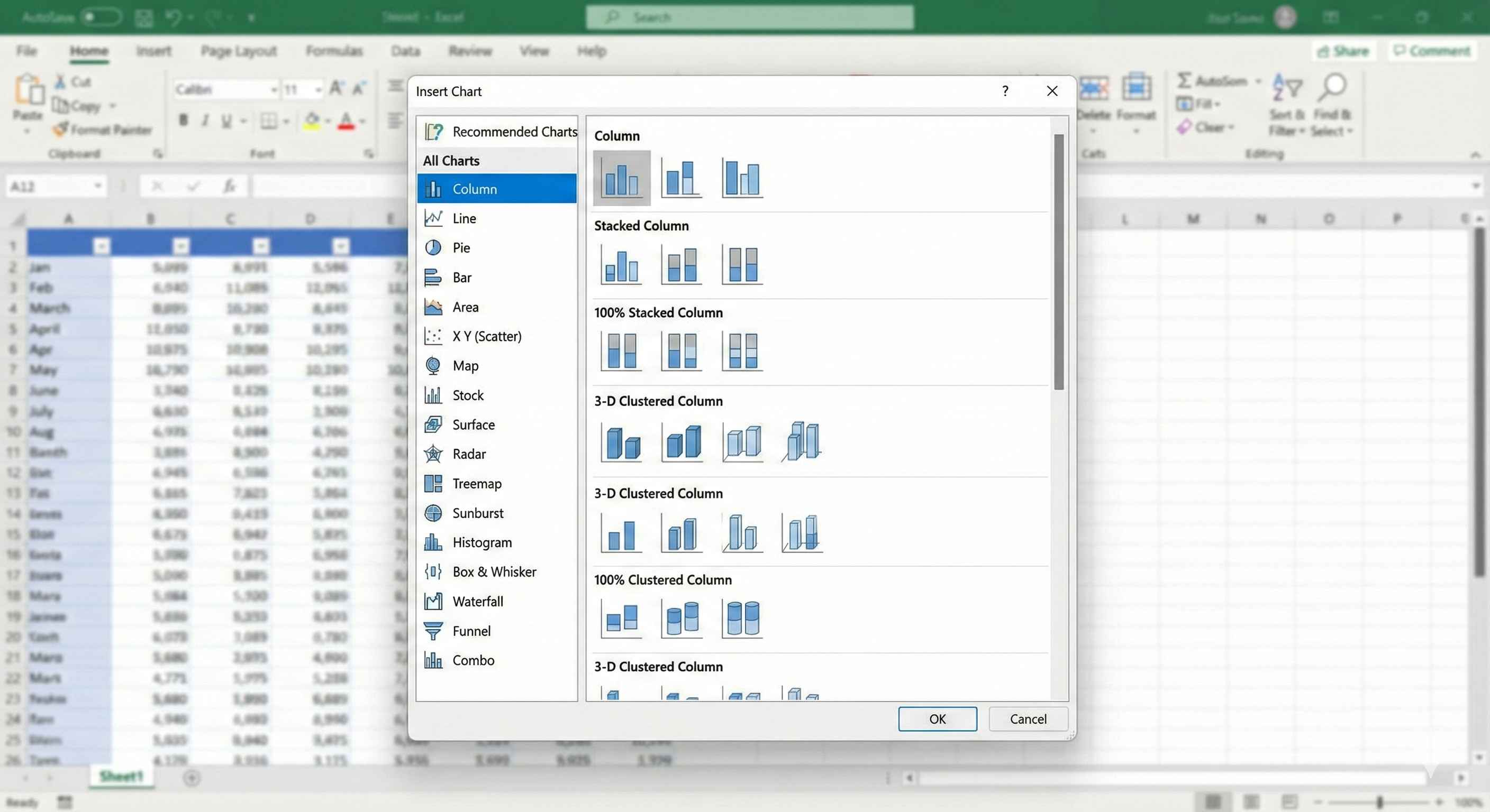
Step 2: Go to Insert tab
Step 3: Click PivotChart
Step 4: Choose a chart type (Column is most common)
Step 5: Click OK
Your chart appears next to the PivotTable.
Choosing the Right Chart Type
| Chart Type | Use When | Example |
|---|---|---|
| Column | Comparing categories | Sales by Product |
| Bar | Long category names | Sales by Salesperson |
| Line | Showing trends over time | Monthly Revenue |
| Pie | Showing parts of whole | Market Share |
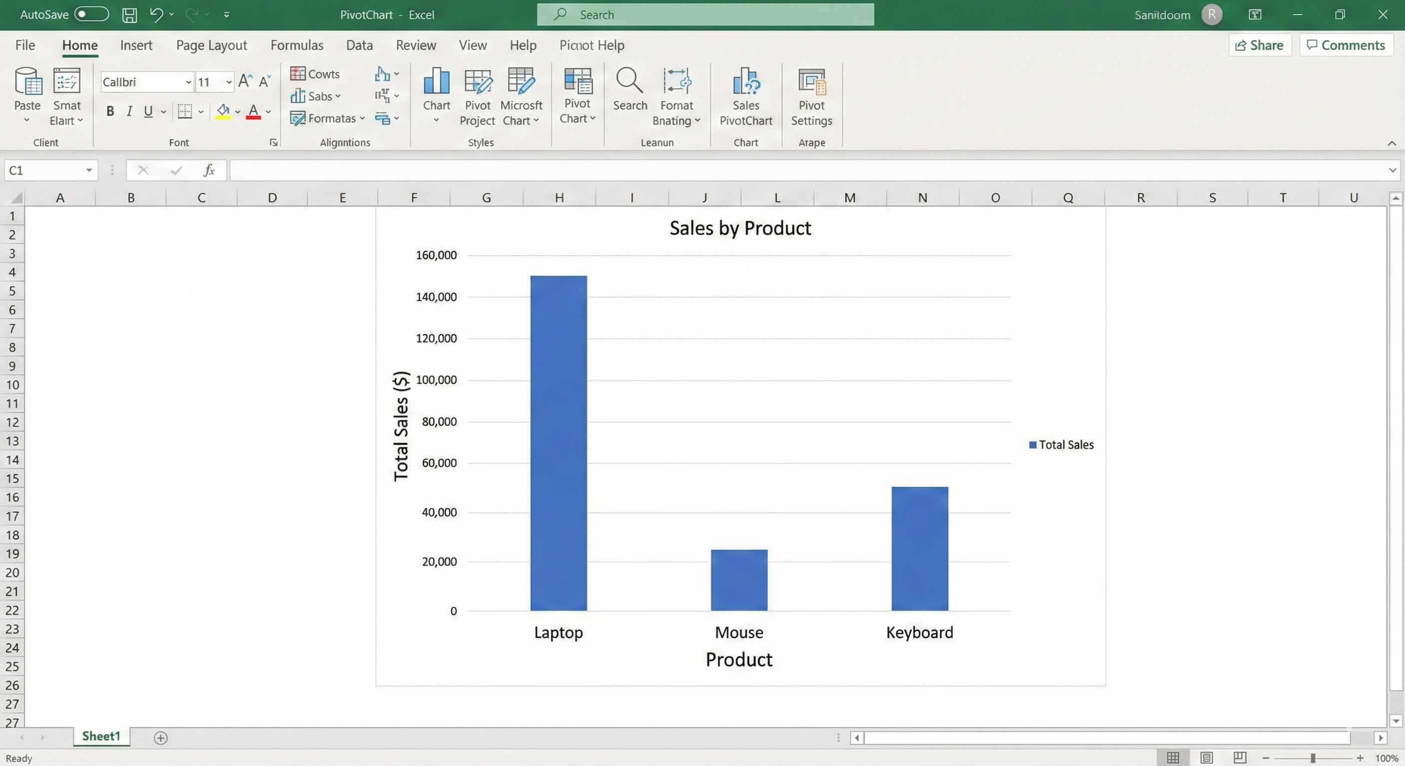
Example: Column Chart
You have a PivotTable showing sales by product:
| Product | Total Sales |
|---|---|
| Laptop | 50000 |
| Mouse | 5000 |
| Keyboard | 8000 |
Create a column chart. You will see three bars. The tallest bar is Laptop (highest sales).
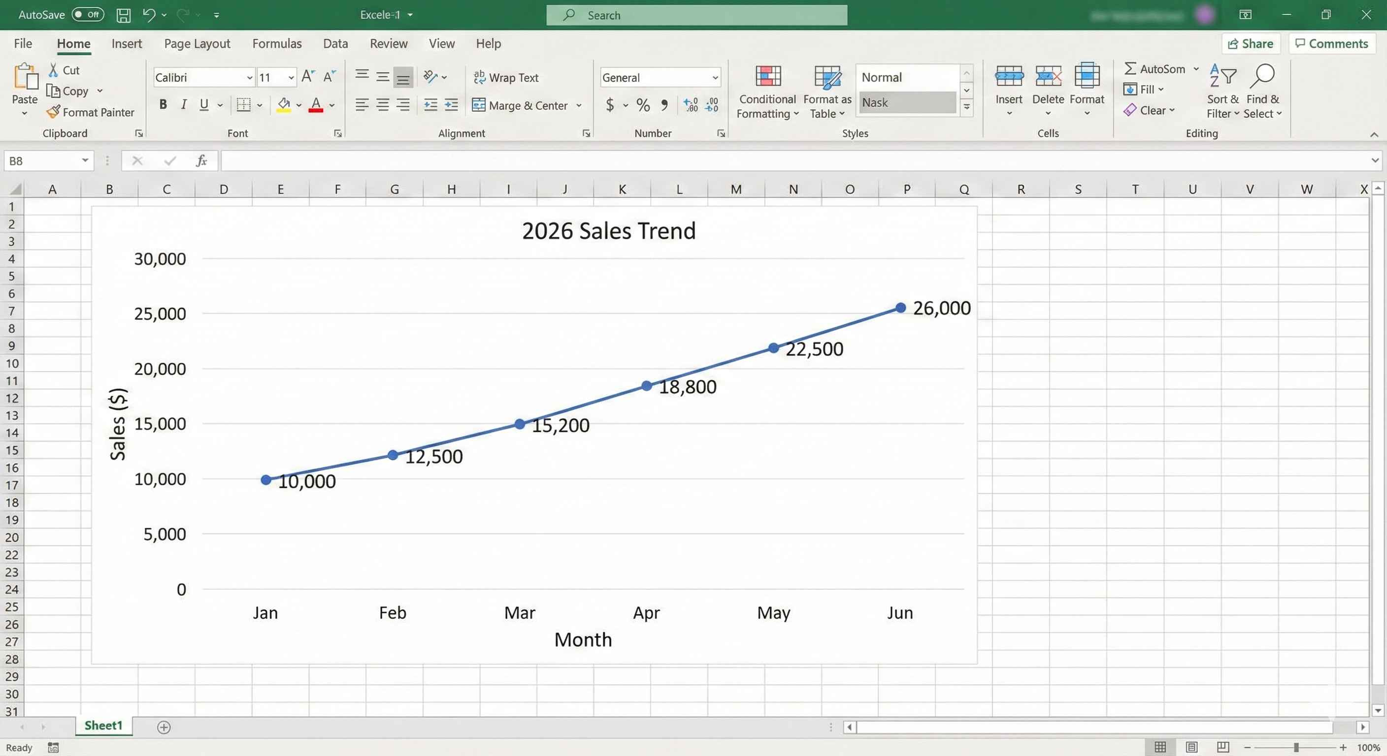
Example: Line Chart
You have monthly sales data.
A line chart shows the trend. You can see if sales are going up, down, or staying flat.
Use line charts when time is involved (days, months, years).
Example: Pie Chart
You want to show what percentage each product contributes to total sales.
Pie chart shows slices. Bigger slice = more sales.
Only use pie charts when you have a few categories (5 or less).
Making Your Chart Look Better
Add a Title:
- Click the chart
- Click the title at the top
- Type a descriptive name like "2024 Sales by Product"
Show Numbers on Bars:
- Click the chart
- Click the + button (top right of chart)
- Check "Data Labels"
Now numbers appear on each bar.
Change Colors:
- Click the chart
- Go to Design tab
- Click Change Colors
- Pick a color scheme you like
The Best Part: Auto-Update
When you change your PivotTable, the chart updates automatically.
- Add a filter to PivotTable? Chart updates.
- Refresh data? Chart updates.
- Change rows or values? Chart updates.
No need to create a new chart.
Filtering Your Chart
PivotCharts have filter buttons on them.
Click the dropdown arrow on the chart to filter what data shows.
Example: Your chart shows all regions. Click the filter and select only "East". Now the chart shows only East region data.
Common Mistakes
Mistake 1: Using pie chart for too many categories Solution: Use column chart if you have more than 5 categories
Mistake 2: No title on chart Solution: Always add a descriptive title
Mistake 3: Wrong chart for data type Solution: Use line for trends, column for comparisons, pie for percentages
Tips for Good Charts
- Keep it simple. Remove unnecessary lines and decorations.
- Use clear titles. "Sales by Product 2024" not "Chart 1".
- Choose colors that are easy to read.
- Do not use 3D effects. They make charts harder to read.
Moving and Resizing
Move: Click and drag the chart to a new location
Resize: Click the chart, then drag the corners
Move to New Sheet: Right-click chart > Move Chart > New Sheet
Summary
- PivotCharts visualize PivotTable data
- Insert tab > PivotChart
- Column chart for comparisons
- Line chart for trends over time
- Pie chart for parts of a whole (5 or fewer categories)
- Charts update automatically with PivotTable
- Add titles and labels for clarity
Charts make your data come alive. Use them in reports and presentations.