Financial Model - Phase 3: Analysis & Metrics

Great progress! You now have 12 months of projections. Let's add analysis.

Phase Progress

✅ Phase 1: Setup & Inputs ✅ Phase 2: Calculations Engine 🔵 Phase 3: Analysis & Metrics (You are here)

• Phase 4: Dashboard & Polish

Step 7: Add Summary Metrics

Let's calculate important business metrics at the top.

Instructions:

1. Add summary section in the Calculations sheet:

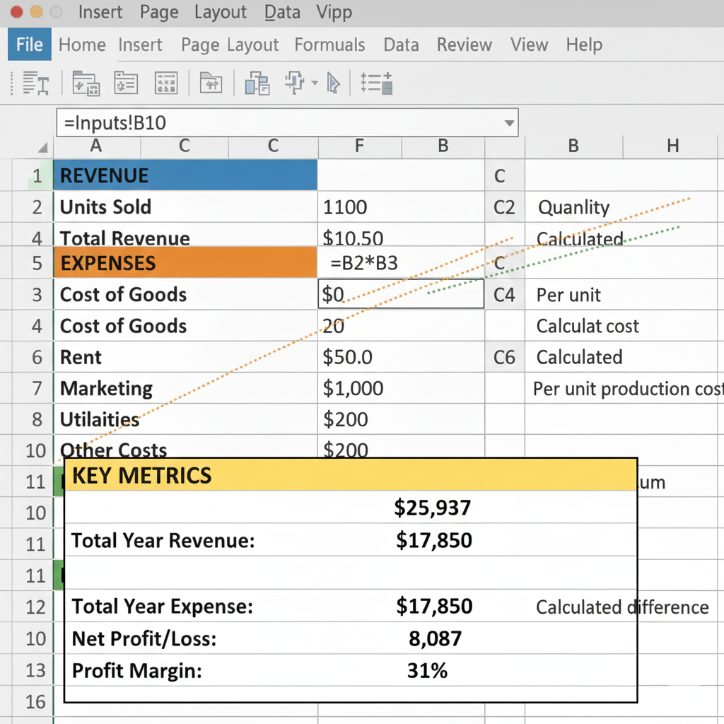
   • Cell A18: Type "KEY METRICS"
   • Make it Bold + Yellow background

2. Calculate total revenue for the year:

   • Cell A19: Type "Total Year Revenue:"
   • Cell B19: Type =SUM(B6:M6)
   • Result: around $25,937

3. Calculate total expenses:

   • Cell A20: Type "Total Year Expenses:"
   • Cell B20: Type =SUM(B14:M14)

4. Calculate net profit:

   • Cell A21: Type "Net Profit/Loss:"
   • Cell B21: Type =B19-B20

5. Calculate profit margin:

   • Cell A22: Type "Profit Margin:"
   • Cell B22: Type =B21/B19
   • Format as percentage (Ctrl + Shift + %)

✓ Checkpoint: Your summary should show:

• Total Revenue: ~$25,937
• Total Expenses: ~$17,850
• Net Profit: ~$8,087
• Profit Margin: ~31%

Step 8: Find the Break-Even Month

When do we start making money? Let's find out.

Instructions:

1. Add Break-Even section:

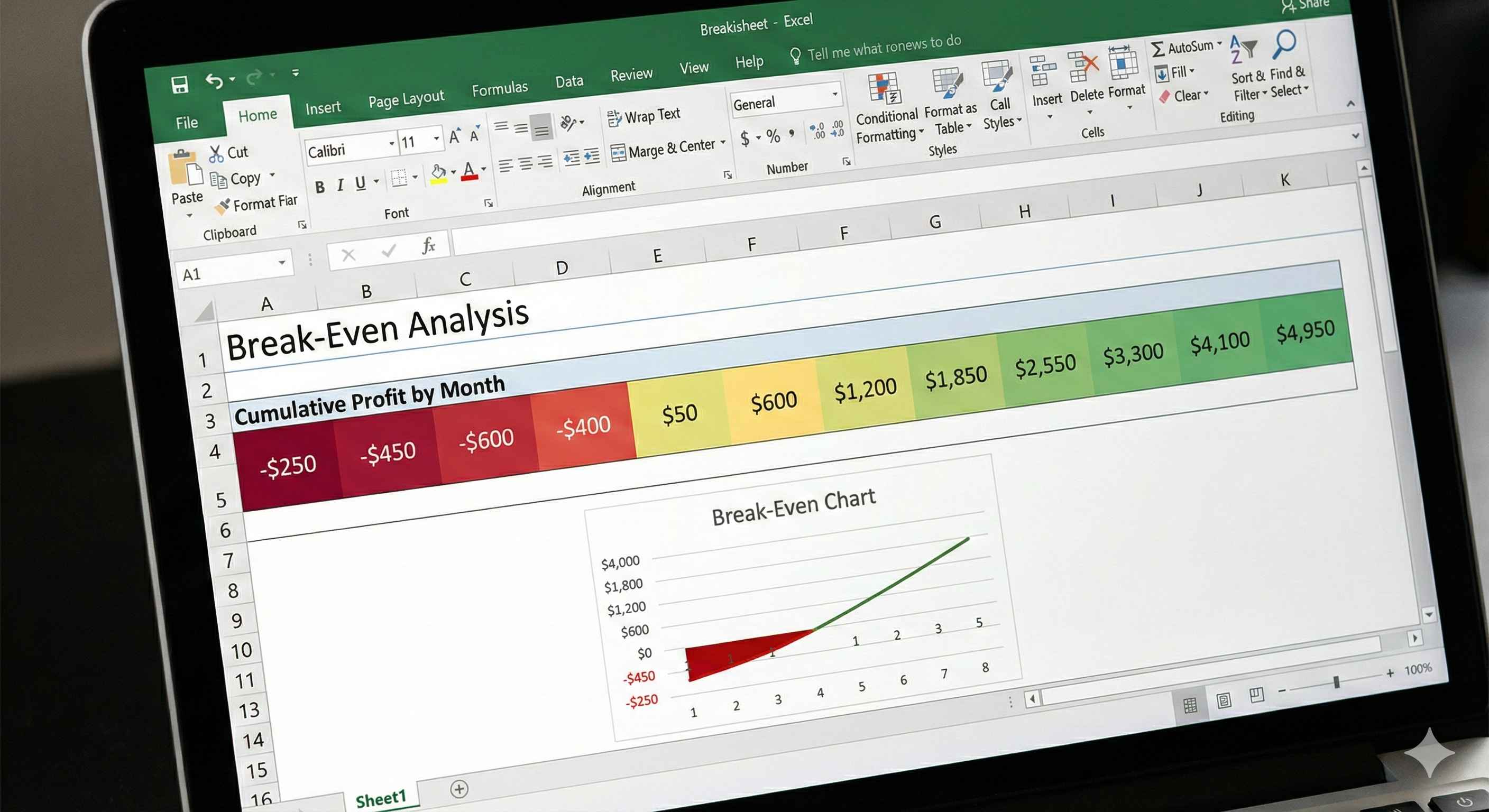
   • Cell A24: "BREAK-EVEN ANALYSIS"
   • Cell A25: "Cumulative Profit by Month:"

2. Calculate cumulative profit (running total):

   • Cell B25: =B16 (Month 1 profit: -$250)
   • Cell C25: =B25+C16 (Previous cumulative + current month)
   • Copy C25 right to M25

This creates a running total. When it goes positive, you've broken even!

3. Highlight the break-even point:
   • Select B25:M25
   • Conditional Formatting → Color Scales → Green-Yellow-Red
   • Green = profitable, Red = still in the red

✓ Checkpoint: Cumulative profit should:

• Start negative (Month 1: -$250)
• Turn positive around Month 4-5
• End at ~$8,087 (same as annual net profit)